
BigQuery is a great data warehouse that lets you quickly and easily search through billions of rows of data in just a few seconds. Both enterprises and startups find it practical and manageable because you can use standard SQL language to query data in BigQuery.
The fully managed data warehouse even comes with a free version and a sandbox version where you can test queries for free. The sandbox version doesn’t even require a credit card to be used. There’s a learning curve that comes with its long list of functions, clauses, and other syntax components, but you don’t need to know everything before you start working with BigQuery.
As experts in BigQuery who build and run data warehouses to make business operations easier, we’ll explain in this comprehensive article how you can use some of the most important window functions in BigQuery. Let’s get started.
What are Google BigQuery Window Functions?
The BigQuery window functions are used to calculate results for a certain group of rows found in tables. The term “window” in the name of these functions might seem a bit odd, but what it actually stands for is a “window of data.” There’s another type of functions known as aggregate functions, which in a way resemble window functions because they’re both concerned with computing data from groups of rows.
The window functions return a certain value for each row, while the aggregate functions return a certain value for all rows (more on this below). Using the window functions, it’s easy to get rid of duplicates or keep track of the totals in a set of rows or a subset of rows.
You’ll probably come across window functions as analytics functions as well. Both terms mean the same. Learning how to use them can help unlock the full power of your data. But first, let’s define these types of functions and what they actually do.
Why Use BigQuery Window Functions?
With BigQuery’s window functions, it’s very easy to find useful data in your tables by filtering them. As long as this data has a common denominator or is of a similar format, you can always make calculations on it and extract useful metrics from it. The window functions can be used in many different ways that depend on the user. But some of the main general use cases are:
- Calculating moving averages,
- Calculating changes between data in rows,
- Calculating totals and deriving cumulative values,
- Ranking data rows based on groups or by certain criteria, etc.
Being that BigQuery has a versatile syntax, there are other functions that can be used to perform similar tasks. For instance, aggregate functions are seen as closely similar to window functions, so it’s important to clarify the distinction between the two.
BigQuery Window (Analytic) vs Aggregate Functions
Aggregate functions are employed to calculate the sum of a group of rows and then return a single value at the end. On the other hand, window functions are used to calculate the value of one or multiple rows while displaying a new result for each row.
Another major difference between the two types of functions lies in their syntax. Window functions are characterized by the clause OVER. All the other functions that seem similar to the window functions but don’t have the OVER clause are either aggregate or scalar functions.
You can also preserve rows of data when using window functions, but you cannot achieve the same with aggregate functions.
BigQuery Window Functions Syntax
BigQuery offers a wide variety of functions that can be used to filter through datasets and extract valuable insights. The window functions are frequently used for this, too.
The window functions syntax is as follows (sourced from Google’s official documentation):
function_name ( [ argument_list ] ) OVER over_clause
over_clause:
{ named_window | ( [ window_specification ] ) }
window_specification:
  [ named_window ]
  [ PARTITION BY partition_expression [, ...] ]
  [ ORDER BY expression [ { ASC | DESC }  ] [, ...] ]
  [ window_frame_clause ]
window_frame_clause:
{ rows_range } { frame_start | frame_between }
rows_range:
{ ROWS | RANGE }
However, looking at the syntax alone is not enough to understand the functions thoroughly. That’s why we’ve provided examples below to further explain how the functions work.
BigQuery Window Function Parameters and Notation Standards
The window functions seem hard to understand, so here’s a breakdown of all the clauses based on the brackets that surround them:
- [] – optional clauses.
- () – actual parentheses.
- | – presence of a logical OR.
- [, … ] – a list of comma-separated items that .
- {} – a group of options.
The OVER clause makes the window functions notably different from other functions. That’s where you define the set of rows (a window frame) that you want to compute results for. The OVER keyword is used when writing queries in Standard SQL as one of the many differences in syntax between Legacy SQL and Standard SQL.
List of BigQuery Window Functions
Whether you’re searching for a function to calculate the moving averages or percentiles or to find a particular value within a dataset, the long list of window functions offers many options. These functions are mainly separated into three categories:
Aggregate BigQuery Functions
Didn’t we just state that analytic (window) functions are different from aggregate functions? Yes, that’s true. But we can still build window functions if we use the OVER clause in our function and complement it with the aggregate functions.
| Function | Explanation |
| ARRAY_AGG | Outputs an array consisting of the values in the windowed rows. |
| SUM | Outputs the sum of non-NULL values for a selected range. |
| ANY_VALUE | Queries through the windowed rows and outputs a random row. |
| CORR | It gives the Pearson coefficient for these two values by using the first number as a dependent variable and the second number as an independent variable. |
| AVG | Outputs the average of the windowed rows (always for non-NULL values) |
| COUNT | Outputs the number of rows for the inputted range. |
| COUNTIF | Outputs the number of rows for the group of rows that respect a certain expression. |
| COVAR_POP | Outputs the population covariance for the inputted pairs. |
| COVAR_SAMP | Outputs the sample covariance for the inputted pairs of numbers. |
| MAX | Outputs the maximum value for the given non-NULL expressions. |
| MIN | Outputs the minimum value for the given non-NULL expressions. |
| ST_CLUSTERDBSCAN | Outputs a DBSCAN clustering for a selected column of geographies. |
| STDDEV_POP | Outputs the population standard deviation for the selected values. |
| STDDEV_SAMP | Outputs the sample standard deviation for the selected values. |
| STRING_AGG | Outputs the concatenation of the selected non-NULL values as a STRING value. |
| VAR_POP | Outputs the population variance for the selected values. |
| VAR_SAMP | Outputs the sample variance for the selected values. |
As the main verb for these types of functions signifies, all of them involve performing some kind of addition with the selected values.
Now, let’s have a look at the second type of window functions, which are navigational functions.
Navigational BigQuery Functions
The navigational functions focus on computing a particular part of the data over a different row in the selected window frame from the present row.
| Function | Explanation |
| FIRST_VALUE | Outputs the value of the initial row found in the current window frame. |
| LAST_VALUE | Outputs the value of the end row found in the current window frame. |
| NTH_VALUE | Outputs the value of the nth row found in the current window frame. |
| LEAD | Outputs the value of the subsequent row in the current window frame after having determined an offset for it. |
| LAG | Outputs the value of the preceding row in the current window frame after having determined an offset for it. |
| PERCENTILE_CONT | Outputs the percentile value with linear interpolation for a group of windowed values. |
| PERCENTILE_DISC | Outputs the percentile value for a group of discrete values. |
| Note: Even though the syntax for the navigational functions (especially the syntax of the OVER clause) could vary, the data type of the result is always the same. |
Numbering BigQuery Functions
The numbering functions, which are the third type of window functions, assign integer values to the existing rows according to their position within the selected window.
| FUNCTION | Explanation |
| ROW_NUMBER | Outputs the sequential row integer for each selected partition. |
| RANK | Outputs the rank for each row in the ordered partition, starting from 1. |
| DENSE_RANK | Outputs the rank for each row within the window partition, starting from 1. |
| PERCENT_RANK | Outputs the percentile rank of a specific row in a particular partition. |
| CUME_DIST | Outputs the relative rank of a row in a selected partition. |
| NTILE | Outputs the respective bucket number after grouping the rows into constant_integer_expression buckets according to the row ordering. |
BigQuery Window Functions Examples
So far, we’ve explained 30 window functions that you can start using immediately. But that might be hard without first seeing some real-life examples. That’s why we’ve built a table within our dataset in the BigQuery Sandbox and ran six essential window functions in BigQuery.
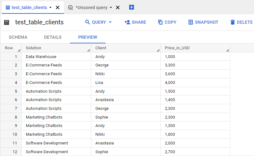
Example table with client data
MAX and MIN BigQuery Examples
Initially, we’ll start off with the MIN function. The function is expected to return the minimal values within the partitions. The syntax is quite simple:
MIN BigQuery Syntax:
MIN(expression) [OVER (...)]
The complete query for our table would be:
SELECT
  Solution,
  Client,
  Price_in_USD,
  MIN(Price_in_USD) OVER (PARTITION BY Client) AS Lowest_package_first
FROM
  `acuto-bigquery.clients.test_table_clients`;
Now, let’s execute this function on the table we created.

Running a MIN function in BigQuery
As expected, the query partitioned the data by client and ranked the price rows from lowest to highest.
Now, let’s test out the MAX function, which is supposed to return the opposite (the maximum values).
MAX BigQuery Syntax:
MAX(expression)[OVER (...)]
The query for this case has only been slightly modified compared to the previous one.
SELECT
  Solution,
  Client,
  Price_in_USD,
  MAX(Price_in_USD) OVER (PARTITION BY Client) AS Highest_package_first
FROM
  `acuto-bigquery.clients.test_table_clients`;
Let’s see how it works in practice:
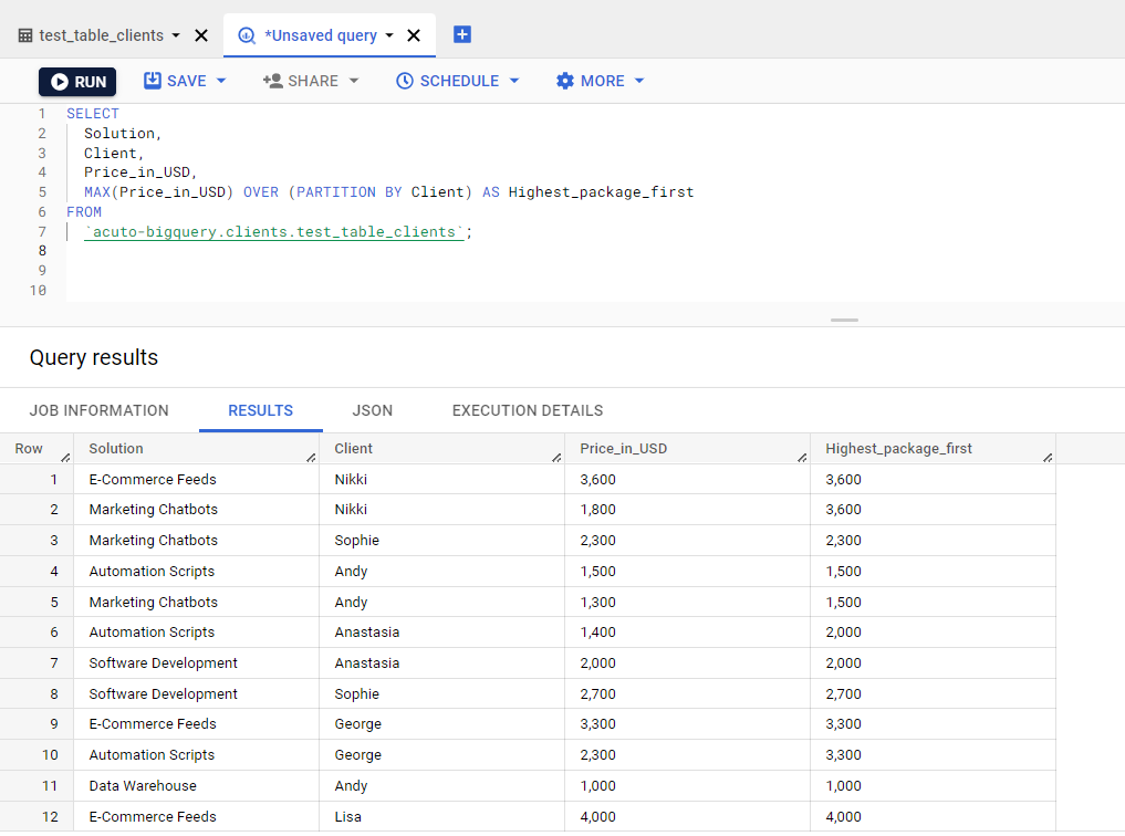
Running a MAX function in BigQuery
As expected, the rows are ordered by price from most expensive to least expensive, with the most expensive solutions for each partition at the top.
LAG and LEAD BigQuery Examples
Operations done on datasets can be very different, and sometimes you may need to know what values came before and after each row. That’s what the LAG and LEAD functions in BigQuery do, as we also explained in the table about navigational functions above.
So, let’s start with the LAG function. We’ll use the same table as we did with the MIN and MAX examples.
LAG BigQuery Function Syntax
The LAG function provides the values of the preceding row of the specified row. Its syntax looks like this:
LAG (value_expression[, offset [, default_expression]])
Now let’s write a query to execute on our table. Using the rules, the query would look like this:
SELECT
  Solution,
  Client,
  Price_in_USD,
  LAG(Price_in_USD,1) OVER (PARTITION BY Solution ORDER BY Price_in_USD) AS Previous_solution
FROM
  `acuto-bigquery.clients.test_table_clients`;
Now, let’s run the query and see what it outputs:
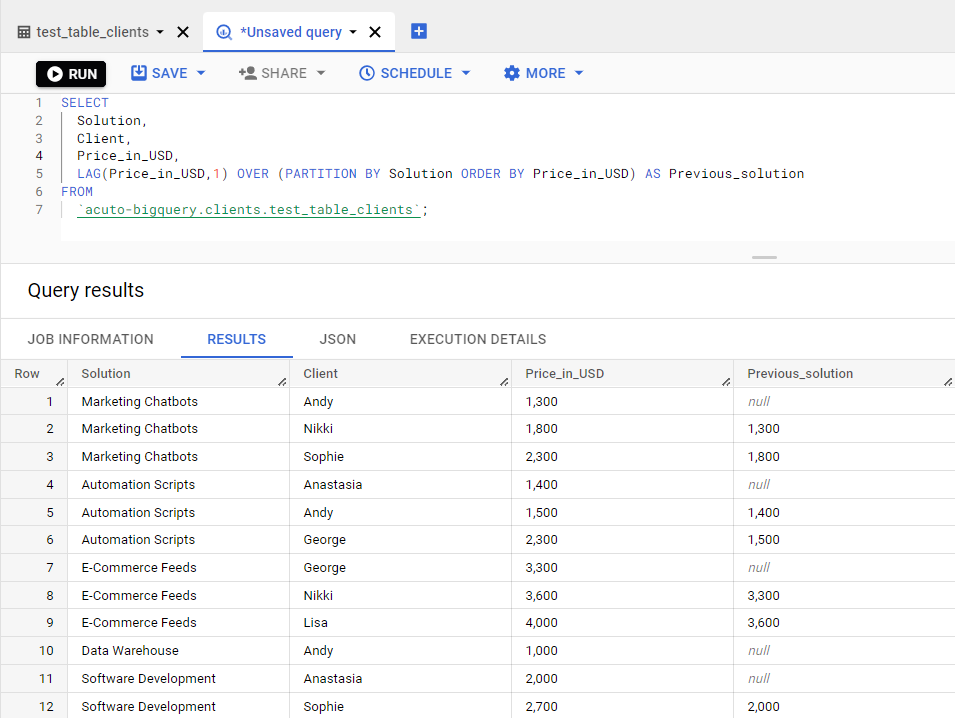
Running a LAG function in BigQuery
The query returned a column pointing at the previous solution, as expected.
LEAD BigQuery Function Syntax
The LEAD function does the opposite of the LAG function. It outputs the subsequent row coming after the specified row. The syntax is quite similar to the LAG function syntax:
LEAD (value_expression[, offset [, default_expression]])
The changes we need to make in the syntax are quite minimal here, too. Our query for this example would be:
SELECT
  Solution,
  Client,
  Price_in_USD,
  LEAD(Price_in_USD,1) OVER (PARTITION BY Solution ORDER BY Price_in_USD) AS Previous_solution
FROM
  `acuto-bigquery.clients.test_table_clients`;
Now, let’s run this query and see what it outputs:
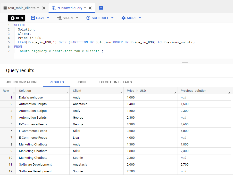
Running a LEAD function in BigQuery
RANK and NTILE BigQuery Examples
These are two of the most commonly used numbering functions in BigQuery. They assign ranks to rows based on the value of rows within the partitions.
RANK BigQuery Function Syntax
The rank function doesn’t require any specific conditions. Therefore, its syntax is simple:
RANK() OVER clause
If we were to write a query for our table, it would appear like this:
SELECT
Client,
Solution,
Price_in_USD,
RANK() OVER (PARTITION BY Client ORDER BY Price_in_USD) AS Project_Nr
FROM
`acuto-bigquery.clients.test_table_clients`;
Now, let’s see what results it produces:

Running a RANK function in BigQuery
Each one of the rows is being assigned a number, cumulating the number of projects for each client.
What about the NTILE function? Let’s have a look at it.
NTILE BigQuery Function Syntax
The NTILE function is similar to the RANK function since it assigns ranks to rows within partitions, but with a slight difference: it packs the rows into nearly similar-sized buckets. Its syntax looks like this:
NTILE(constant_integer_expression) OVER over_clause
Our query for this example would be:
SELECT
Solution,
Price_in_USD,
NTILE(5) OVER (PARTITION BY Solution ORDER BY Price_in_USD) AS Buckets
FROM
`acuto-bigquery.clients.test_table_clients`;
Now, let’s run it and see the results that it outputs:

Running an NTILE function in BigQuery
Conclusion
Writing queries in BigQuery can be daunting if you don’t have extensive SQL knowledge in order to produce the results that you want to extract from your data. In this article, we’ve explored some of the most commonly used window functions in BigQuery used for this purpose.
These analytic (window) functions are divided into three main subsets: numbering, navigational and aggregate functions. Each of them yields particular information from your datasets.
However, their syntax could take hours to master. But you can avoid spending countless hours writing these queries to just generate a few reports.
We can build a data warehouse and manage it for you while you spend your time on tasks that are hard to automate. Furthermore, if you want to save more time by automating other time-consuming daily tasks, Acuto can build customized automation scripts for you.
Schedule a call with our team in less than a minute to learn more about our services!